Software for new tomography device

Scientists from Tomsk State University have created a microtomography device which can provide data about the inner structure of various materials, such as diamonds, to an accuracy of one micron. But, examining a fly stuck inside the device might be more interesting.

EDISON Software Development Centre was asked to create the software for a microtomography device. The article ‘How does one develop software for a microtomography device in 5,233 man-hours’, gave an overview of how this was achieved, detailing algorithms, mathematical solutions, the implementation and the debugging process.

Nevertheless, insatiable readers assailed us with questions, to which we have now, finally, responded below...

The tomograph can scan matter with a resolution of up to one micron. That is, one hundred times thinner than the width of a human hair. Once a scan has been completed, the program creates a 3D model, which shows not only the external form of the object but also its internal structure.

General technical specifications

X-Ray emitter

• Voltage: 20–160 kV
• Amperage: 0–250 µA
• Wattage: 10 W
• Focal spot diameter: 1–5 µm

X-Ray detector based on a CCD-matrix

• CCD sensitive area dimensions: 2,048 × 2,048 pixels
• Geometrical pixel size: 13 × 13 µm
• Geometrical size of the CCD sensitive area: 27.6 × 27.6 mm
• Inbuilt two-speed A/D converter (16-bit 100 kHz & 16-bit 2 MHz)

Positioning system

Rotor travel:

• SEMM (Segment Electro-mechatronic Movement Module) – 360°
• LEMM (Linear Electro-mechatronic Movement Module) – 100 mm

Positioning precision, no less than: ±0.5 µm.

Rotor travel speed: from 0.01 up to 20 mm/sec.

Wattage (at an input voltage of 70 V): 0.7 kW.

Questions and answers

Question #1. I'd be interested to read about how the inverse Radon transform is implemented using a point source, as well as the role of CUDA in this.

Radon transform calculations for a point source, if described in diagrammatic form, are similar to those for the parallel mode. In this case, however, the rays are not parallel, which affects the coordinates of points within the cube of the object where densities are to be added. Looking at the transform as a whole, there is not a great difference, from the point of view of the reconstruction, between the different algorithms available. The only thing that changes is the coordinates of line-segments, or rays, and the formulae for their calculation.

Furthermore, when on the basis of shadow projection, we have obtained rays from the source to every point of the projection in the coordinate space of the microtomograph, and we know the position of the rotating cube of the object, the voxels along each ray can be calculated. Each voxel is assigned a pixel density value from the shadow projection, corresponding to the density at which it is penetrated by the ray from the source; the data type of their masses is then converted to float. Finally, for every shadow projection, we repeat the same operation of projecting onto the voxels, taking into consideration the angle of projection. After this, all aggregate values of voxels are normalised to the bit depth in which they are going to be stored later – usually this is 16-bit unsigned integer. This description explains, in an extremely simplified way, the process of reconstruction and acquisition of the final voxel model. A more detailed explanation of this algorithm follows.

An x-ray system generates a flat shadow image of the whole inner volumetric structure of the sample. However, in a single shadow projection, the depth distributions of the sample's structures blend together completely. Only x-ray tomography allows for the visualisation and the measurement of dimensional structures of samples without chemical or mechanical processing.

Any x-ray shadow image is a flat projection of a 3D object. In the simplest of cases, it can be described as an image received from parallel x-rays. In this approximation, every point of the shadow image contains the aggregate information about the absorption of a particular x-ray beam through the entire volume of the 3D object. Due to the parallel geometry of x-ray beams, the reconstruction of a 3D image, from the sample of a 2D shadow projection, is achieved by means of reconstructing a series of 2D cuts of the original along the 1D shadow lines. The possibility of carrying out reconstructions of this kind can be demonstrated with a very simple example. Let us consider an object with a single point, with high adsorption at an undefined location.

On a 1D shadow line, we will see a decrease in intensity resulting from its absorption into an adsorbing object. Now, in the computer's memory, we can model an empty row of pixels (image elements) corresponding to the supposed shift of the object. Needless to say, we should make sure that all parts of the reconstructed object are within view. Since we know the location of the shadows from the absorbing areas of the object, we can use the reconstructed area in the computer's memory to define all possible positions of absorbing areas inside the object in the form of lines. Now we can start rotating the object and repeating the same operation. In each new position of the object, we will add to the reconstructed area lines of possible positions of the object judging by the position of its shadow projections. This operation is called back projection. After several rotations, we can isolate the position of the absorbing area inside the reconstructed range. With an increase in the number of shadow projections made from different directions, the localisation becomes more and more precise.

With a reconstruction based on an infinite number of projections, we can obtain an image with a good precision of absorbing area position identification inside the object under observation. At the same time, however, the dot pattern will have a blurred area around it, since it was received as a result of the overlapping of lines with various possible deviations. Now, since we know that the image was formed by a point object, we can conduct a preliminary correction of the initial information within the adsorption lines to make the final image more consistent with the real object. This correction adds a certain amount of negative adsorption along the outer border of the point to eliminate the diffusing characteristic of the back-projection process. This algorithm provides not only images of sections of separate point structures but allows for the study of real objects. Every material object can be viewed as a great number of separate elementary absorbing volumes, and the linear adsorption in each x-ray beam corresponds to the aggregate adsorption on all absorbing structures encountered by the beam.

Two-dimensional sections of an object can therefore be reconstructed from 1D shadow lines received from various perspectives. Most x-ray emitters cannot, however, generate parallel radiation beams. In reality, point-like sources are used to generate cone beam x-rays.

In fan-beam geometry, the reconstructed sections will have some distortions in the areas more distant from the optical axis of the beam. To solve this problem, we need to use an algorithm for 3D cone beam reconstruction (Feldkamp–Davis–Kress Algorithm) in order to take the thickness of the object into consideration. In other words, the rays which penetrate the front and the back surfaces of the object will not be projected in the same row as the detector. Thus, the fastest section to reconstruct is the central section, since it does not require any image correction to account for the thickness of the object.

For the x-ray examination of an object, the image contains information about the reduced intensity of incident solar radiation inside the object. Since the absorption of x-rays is expressed in exponential form (the Beer–Lambert law), linear information about the adsorption of radiation from the shadow projection can be obtained using a logarithmic function. Given that a logarithm is a nonlinear operation, even the slightest noise in the signal can result in serious errors during the reconstruction phase. To avoid such errors, initial data averaging can be used. On the other hand, we could try to enhance the signal noise in relation to the shadow image by optimising the exposure time to gain more representative information. The most effective way of reducing noise in the process of reconstruction is through a correct choice of a correction/filtering function for convolution, taking place before back projection. In the simplest (abovementioned) case, the correction function produces two reactions of negative adsorption around any signal or noise peak in the shadow line, but such behaviour becomes rather risky when working with a noisy channel. This problem can be solved by choosing the convolution function with spectral limitations (the Hamming window).

Outline of CUDA and the reconstruction process

Data reconstruction from shadow projections

The maximum size of the reconstruction cube is 1,024 × 1,024 × 1,024 voxels. We shall describe a cube of such volume as an elementary cube. The algorithm allows for the reconstruction of smaller cubes, but the dimensions in all directions should be divisible by 32. In one run, the cube layer should not be more than 128 Mb, i.e. 1/8 of an elementary cube, is reconstructed. If there are several CUDA devices installed in the system, then the reconstruction process will be run on them simultaneously.

Shadow projections are loaded onto the RAM drive during the first run, in the amounts sufficient for the reconstruction of the cube. For example, if the reconstruction of the cube requires 1,200 lines from the shadow projection, but the file limit is 2,000, only the required 1,200 will be uploaded onto the RAM and cached. Since it is very likely that the segments of projection will overlap in the process of the next cube reconstruction, we can use the data, which has already been uploaded, one more time, only then having to upload the new lines.

Connecting to the server and task distribution

Broadcasting of UDP packets is used to find clients and servers. The server sends out a notification upon start-up and subsequently sends notifications at five-minute intervals. The client, when launched, sends out a broadcast query which, in turn, sends out an immediate server response command. The client, having received a notification about an available server, connects to it via TCP, which is used to send executive commands and tasks and receive reports about task termination. All clients, servers and tasks have unique identifiers.

When the connection to one of the servers is lost, the server is considered to have stopped, and its tasks are distributed among the others. When a new server is connected, the tasks are neither taken away from other servers nor redirected towards it. That is why, to provide an even load, it is very important to find all servers before the start of reconstruction task distribution. As more cubes are being made ready, it becomes possible to launch integration tasks. These tasks are directed to a random server. The tasks of reconstruction and integration are performed by servers simultaneously.

Tasks may come from several clients. The server processes them in order of their appearance (FIFO). The client operates best when sending out reconstruction tasks from one layer of elementary cubes to one server. This is to reduce the amount of data necessary for the server to begin reconstruction. The amount of server RAM determines the strategy of reconstruction and compression of cubes. If there is a large amount of memory, (more than 20 GB) then the compression of the previous cube and the reconstruction of the next one is done simultaneously, otherwise the reconstruction of the next cube will not start until the previous one has been fully processed, i.e. compressed and saved to the hard drive.

The main stages of reconstruction

First of all, projection segments, into which the reconstructed volume is being projected, are determined after accounting for perspective. The projections needed for reconstruction are identified on the basis of this data. If the RAM cache contains segments of files that are not on this list, they will be deleted from the memory.

The reconstruction thread addresses the cache for a segment of the projection, the memory unit containing the projection (considering the page size of 4,096 bytes) has its memory locked, which prevents it from being replaced, and the pointer is passed along to the CUDA procedure. All of the following operations are held in the memory of the accelerator. First of all, the 12-bit storage format is decompressed into a float data type, and all further calculations are conducted in float. During decompression, the segment is trimmed on both the left and right to fit the length of the reconstructed block, with some allowance for convolution when filtering the projection. Some preliminary processing is conducted: inversion, gamma-correction, filtering by averaged projection, and conducting the necessary number of smoothing iterations. Then, the convolution is carried out and the segment again is trimmed on the left and on the right to the minimum width needed for back projection. In this way, the projections are processed until there is no free memory on the video card. Thus, an array of segments ready for back projection is formed.

The essence of back projection lies in summing the weights of all the x-ray projections of a particular point for every voxel. One CUDA-core request manages calculations for 32 voxels placed one above the other. At the same time, a cycle is made through all projection segments uploaded to the memory. This allows for the storage of all intermediate data in registers without any intermediary storage. At the end of the calculation stage, the value of the voxel's density is recorded in the memory. The back-projection kernel has two possible implementations. One of them, the slow implementation, includes checks to see if there is a point on the projection to draw data from, since such a point is not necessarily present. The fast implementation does not account for checks. The appropriate implementation is chosen automatically. The selection of a value from the projection is carried out according to the ‘nearest neighbour algorithm’. The use of texture memory, during the early stages, led to a sharp reduction in efficiency. At this stage, when projection arrays were used, it appeared impossible to create texture arrays due to the limitations posed by CUDA 4.2.

If there isn't enough memory, the calculations might need several iterations of projection uploads and back projections. When the calculations are completed, the obtained voxels are evaluated. Maximum and minimum density values are calculated and a bar chart is created. Plotting the bar chart and copying the results onto the RAM drive are done simultaneously.

When there are several CUDA devices, the segments of a reconstructed cube are processed simultaneously. Once the reconstruction of a cube has completed, another thread takes on the task of compressing the cube, and the reconstruction thread immediately undertakes the next task, providing that there is enough RAM capacity. Dedicating and freeing up large segments of memory proved to be a very time-consuming operation, which is why all large already-obtained memory units have been used in subsequent calculations. This is why, some CUDA memory is dedicated to voxels, some for a series of intermediary buffers, and the rest of the memory is allocated to projections. The projection stores are managed manually.

Compression

Compression to octree is conducted in several threads. The number of threads depends on the number of processor cores. Every thread processes its own octant. It is then saved in a file indicated by the task's reconstruction client. A notification is finally sent that the processing of the cube is complete.

Client

The client maintains a database of cubes in the form of an SQLite file. Cube characteristics, reconstruction time and other values are stored there. Upon finishing the reconstruction, the client program closes, and package tasks for reconstruction can be organised.

A sample CUDA code

The core (measureModel.cu) operates the first run while plotting the bar chart. The file is given to demonstrate the general form of CUDA code in an actual working project.

#include <iostream>
#include <cuda_runtime.h>
#include <cuda.h>
#include <device_functions.h>

#include "CudaUtils.h"
#include "measureModel.h"

#define nullptr NULL

struct MinAndMaxValue
{
  float minValue;
  float maxValue;
};
__global__ void
cudaMeasureCubeKernel(float* src, MinAndMaxValue* dst, int ySize, int sliceSize, int blocksPerGridX)
{
    int x = blockDim.x * blockIdx.x + threadIdx.x;
    int z = blockDim.y * blockIdx.y + threadIdx.y;
    int indx = z * blocksPerGridX * blockDim.x + x;
    MinAndMaxValue v;
    v.minValue = src[indx];
    v.maxValue = v.minValue;
    //indx += sliceSize;
    for (int i = 0; i < ySize; ++i)
    {
      float val = src[indx];
      indx += sliceSize;
      if (v.minValue > val)
      v.minValue = val;
      if (v.maxValue < val)
      v.maxValue = val;
    }
    
    //placing of data from our line in a shared memory
    __shared__ MinAndMaxValue tmp[16][16];
    tmp[threadIdx.y][threadIdx.x] = v;
    //all threads of our block have calculated their values
    __syncthreads();

    if (threadIdx.y == 0)
    {//the first line of all threads shall be convolution of temporary data up to 16 values
        for (int i = 0; i < blockDim.y; i++)
        {
          if (v.minValue > tmp[i][threadIdx.x].minValue)
          v.minValue = tmp[i][threadIdx.x].minValue;
          if (v.maxValue < tmp[i][threadIdx.x].maxValue)
          v.maxValue = tmp[i][threadIdx.x].maxValue;
        }
        tmp[0][threadIdx.x] = v;
    }
    __syncthreads();
    ///checking for a particular value 
    if (threadIdx.x == 0 && threadIdx.y == 0)
    {
        for (int i = 0; i < blockDim.y; i++)
        {
          if (v.minValue > tmp[0][i].minValue)
          v.minValue = tmp[0][i].minValue;
          if (v.maxValue < tmp[0][i].maxValue)
            v.maxValue = tmp[0][i].maxValue;
        }
        dst[blockIdx.y * blocksPerGridX + blockIdx.x] = v;
    }
}

void Xrmt::Cuda::CudaMeasureCube(MeasureCubeParams params)
{
//we are going to make calculations for a thread of 256 square blocks
  int threadsPerBlockX = 16;
  int threadsPerBlockZ = 16;
  int blocksPerGridX = (params.xSize + threadsPerBlockX - 1) / threadsPerBlockX;
  int blocksPerGridZ = (params.zSize + threadsPerBlockZ - 1) / threadsPerBlockZ;
  int blockCount = blocksPerGridX * blocksPerGridZ;
  dim3 threadDim(threadsPerBlockX, threadsPerBlockZ);
//grid size

  dim3 gridDim(blocksPerGridX, blocksPerGridZ);

  MinAndMaxValue *d_result = nullptr;
  size_t size = blockCount * sizeof(MinAndMaxValue);
  checkCudaErrors(cudaMalloc( (void**) &d_result, size));

  cudaMeasureCubeKernel<<<gridDim, threadDim>>>(
    params.d_src,
    d_result,
    params.ySize,
    params.xSize * params.zSize,
    blocksPerGridX
  );

  checkCudaErrors(cudaDeviceSynchronize());

  MinAndMaxValue *result = new MinAndMaxValue[blockCount];
  checkCudaErrors(cudaMemcpy(result, d_result, size, cudaMemcpyDeviceToHost));

  params.maxValue = result[0].maxValue;
  params.minValue = result[0].minValue;
  for (int i = 1; i < blockCount; i++)
  {
    params.maxValue = std::max(params.maxValue, result[i].maxValue);
    params.minValue = std::min(params.minValue, result[i].minValue);
  }

  checkCudaErrors(cudaFree(d_result));
}

__global__ void
cudaCropDensityKernel(float* src, int xSize, int ySize, int sliceSize, float minDensity, float maxDensity)
{
  int x = blockDim.x * blockIdx.x + threadIdx.x;
  int z = blockDim.y * blockIdx.y + threadIdx.y;
  int indx = z * xSize + x;
  for (int i = 0; i < ySize; ++i)
  {
    float val = src[indx];
    if (val < minDensity)
        src[indx] = 0;
    else if (val > maxDensity)
        src[indx] = maxDensity;
    indx += sliceSize;
  }
}

void Xrmt::Cuda::CudaPostProcessCube(PostProcessCubeParams params)
{
//we are going to make calculations for a thread of 256 square blocks
  int threadsPerBlockX = 16;
  int threadsPerBlockZ = 16;
  int blocksPerGridX = (params.xSize + threadsPerBlockX - 1) / threadsPerBlockX;
  int blocksPerGridZ = (params.zSize + threadsPerBlockZ - 1) / threadsPerBlockZ;
  dim3 threadDim(threadsPerBlockX, threadsPerBlockZ);
//grid size
  dim3 gridDim(blocksPerGridX, blocksPerGridZ);

  cudaCropDensityKernel<<<gridDim, threadDim>>>(
    params.d_src,
    params.xSize,
    params.ySize,
    params.xSize * params.zSize,
    params.minDensity,
    params.maxDensity
  );

  checkCudaErrors(cudaDeviceSynchronize());
}

//number of parts a unit is divided into
#define DivideCount 8
#define ValuesPerThread 32
#define SplitCount 16
#define SplitCount2 64

__global__ void
cudaBuildGistogramKernel(
  float *src,
  int count,
  int *d_values,
  int minValue,
  int barCount
)
{
//value index, from which we start counting
  int barFrom = threadIdx.x * ValuesPerThread;
  int blockIndx = SplitCount * blockIdx.x + threadIdx.y;
  int blockLen = count / (SplitCount * SplitCount2);

  unsigned int values[ValuesPerThread];
  for (int i = 0; i < ValuesPerThread; i++)
  {
    values[i] = 0;
  }

  src += blockLen * blockIndx;
  for(int i = blockLen - 1; i >= 0; i--)
  {
    float v = src[i];
    int indx = (int)((v - (float)minValue) * DivideCount) - barFrom;
    if (indx >= 0 && indx < ValuesPerThread)
      values[indx]++;
  }

  for (int i = 0; i < ValuesPerThread; i++)
  {
    d_values[blockIndx * barCount + barFrom + i] = values[i];
  }
}

__global__ void
cudaSumGistogramKernel(
  int *d_values,
  int barCount
)
{
//column index, which we add up
  int barIndx = blockIdx.x * ValuesPerThread + threadIdx.x;

  unsigned int sum = 0;
  d_values += barIndx;
  for (int i = 0 ; i < SplitCount * SplitCount2; i++)
  {
    sum += d_values[i * barCount];
  }

  d_values[0] = sum;
}

void Xrmt::Cuda::CudaBuildGistogram(BuildGistogramParams params)
{
  checkCudaErrors(cudaMemcpyAsync(
  params.h_dst, params.d_src, params.count * sizeof(float), cudaMemcpyDeviceToHost, 0
  ));
  //we define the minimum value in the bar chart
  int minValue = (int)(params.minDensity - 1);//for negative values the fraction is dropped, but that is not enough!
  minValue = std::max(minValue, -200);
  //maximum value in the bar chart
  int maxValue = (int)params.maxDensity;
  maxValue = std::min(maxValue, 200);
  //number of columns in the bar chart (the range of 1 is divided by DivideCount part)
  int barCount = (maxValue - minValue + 1) * DivideCount;
  ///making the number of columns divisible by ValuesPerThread
 int x32 = barCount % ValuesPerThread;
  barCount += (x32 == 0) ? 0 : ValuesPerThread - x32;

  ///thread adjustment:
  /// x – each thread calculates 32 columns, i.e. x is proportional to the width of the bar chart
  /// y – we divide the data block by SplitCount parts
  dim3 threadDim(barCount / 32, SplitCount);
  ///grid size, we divide all data by SplitCount2 parts
  dim3 gridDim(SplitCount2);
  ///thus all data is divided block-wise by SplitCount2 * SplitCount parts
  ///every such part will be processed by barCount / 32 threads

  ///we allocate memory for storage of intermediary data
  int *d_values = nullptr;
  ///each block has its own values
  size_t blockValuesCount = SplitCount2 * SplitCount * barCount;
  size_t d_size = blockValuesCount * sizeof(int);
  checkCudaErrors(cudaMalloc( (void**) &d_values, d_size));

  ///processing block by block
  cudaBuildGistogramKernel<<<gridDim, threadDim>>>(
    params.d_src,
    params.count,
    d_values,
    minValue,
    barCount
  );
  ///we add the blocks on GPU
  cudaSumGistogramKernel<<<dim3(barCount / ValuesPerThread), dim3(ValuesPerThread)>>>(
    d_values,
    barCount
  );
  checkCudaErrors(cudaDeviceSynchronize());
  ///we obtain the values of the bar chart
  params.histogramValues.resize(barCount);
  checkCudaErrors(cudaMemcpy(
    params.histogramValues[0],
    d_values,
    barCount * sizeof(int),
    cudaMemcpyDeviceToHost
  ));
  checkCudaErrors(cudaFree(d_values));
  params.histogramStep = 1.0 / DivideCount;
  params.histogramStart = (float)minValue;
}
 

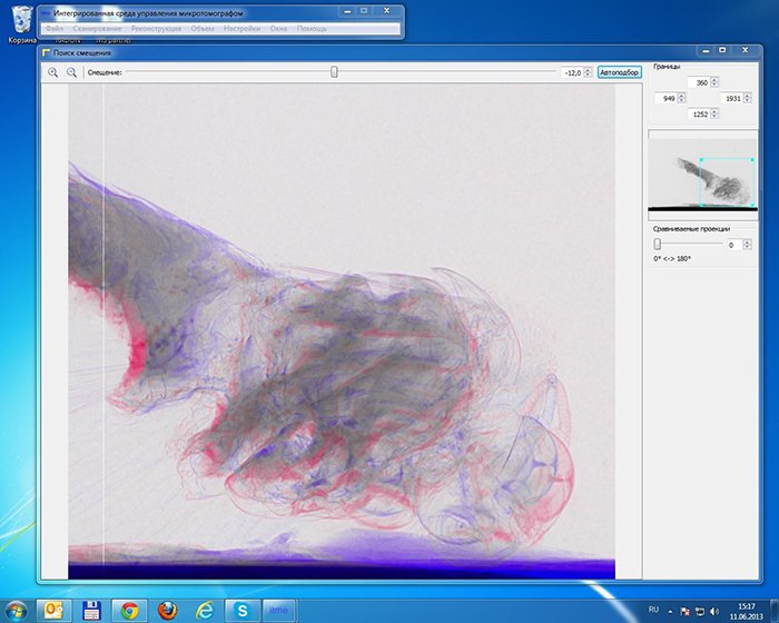
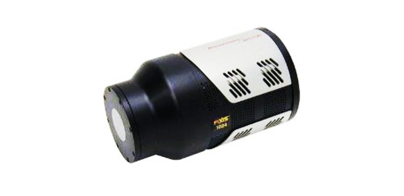
Question #2. The camera that you used (PIXIS-XF, I think) produces 2,048 × 2,048 images. However, in the article you mentioned ‘up to 8,000 × 8,000’. How did you reach this? Are you supposed to move the object, or move the camera vertically and horizontally and later patch the images?

Yes, you are right. The camera used in the microtomograph is the PIXIS-XF: 2048B. The size of the reconstructed image is, according to the requirements, 8,000 × 8,000 × 20,000. 8,000 in width and depth. This means that the camera sees only a part of the image, but the algorithm allows for greater reconstruction by way of many circular projections. Indeed, this accounts for a decrease in quality of the reconstruction along the edges. As for the height, we simply move the table and create a new reconstruction; the results are then patched.

Question #3. Are all the demo images, which are given in the video at the end of the article, received from 360-degree projections? If so, then it's rather good; 360-degree projections in increments of 1 degree are very rare; usually one has to progress in increments of a third or quarter of a degree, otherwise the signs of reconstruction will be visible. I think there was a formula for an optimal number of projections for a specified resolution, but I can't remember it exactly.

In our case, 180–360 projections were used. Various algorithms may provide different reconstruction quality depending on the number of projections, but the rule of thumb is that while the number of projects increase, the quality increases too. For our task, it was sufficient to use 180–360 projections to provide high quality.

The algorithm reacts well to skipped frames at the cost of a slight reduction of resolution in the direction where the gaps are. Besides, the camera had a tendency to get overheated and its ‘brightness’ wavered, which is why some frames were discarded as defective. The others were normalised according to average brightness.

Question #4. I didn't quite understand about the speed of the camera. The specification says that it's dual-frequency 100 kHz or 2 MHz. If it's a four-megapixel camera, does it mean that it shoots a frame every two seconds at the maximum frequency?

Yes, you are correct. According to the camera documentation, its specifications are the following: ADC speed/bits 100 kHz/16-bit and 2 MHz/16-bit.

That means that if one dot of the image has a 16-bit capacity, we will get a frequency for the whole image of 2,000,000 / (2,048 * 2,048) = 0.47 Hz.

Question #5. Do you move the manipulator step by step or continuously? How long does it take to scan the typical samples that were shown in the video?

The manipulator (a table) moves in steps. We turned it around a corner, stopped, made a shot, turned it again etc. The average scanning time was 11 minutes for 378 frames.

Question #6. I'd be interested to learn about the 12-bit setup. It stands to reason that one can cut off four bits and pack each two-pixel unit into three bytes for storage and transferring. But for the reconstruction you will have to expand each pixel into a minimum of two bytes... Or is all of your mathematics based on 12-bit? In that case, how did you solve the problem of the alignment of 1.5-byte pixels in storage?

Here is the file structure for the 12-bit side projections.

1. Pixels are packed bit-by-bit and placed in lines, so that two points take up three bytes; it is being understood that the width of the projection image is divisible by two according to the formula: lineWidthInBytes = width() * 3 / 2.
2. Usually the whole range of data is not loaded at once, but ‘windows’ are used where only the necessary portion of the image is loaded while the left and right borders are supposed to be aligned so as to be divisible by four pixels.
3. After the ‘window’ is loaded further, work is conducted via the function of complete import/export of this window into float or quint16 arrays. During the import/export process, the data is converted from 12-bit to the necessary number of bits.
4. In our case, the benefit from shrinking the size of projection files was greater than the loss of efficiency caused by it. Besides, the entire files were not loaded, instead, the ‘windows’ were, intended to be processed on a particular cluster engine. Indeed, losses in productivity were even smaller thanks to server multitasking.

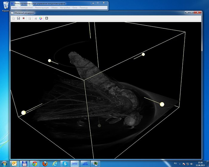
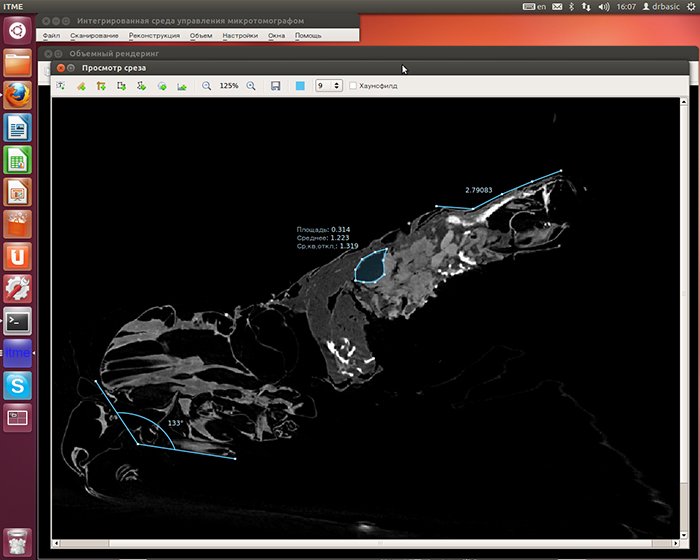
Volume (voxel) rendering in real time

Another interesting task was rendering the model with the use of voxels in real time. Apart from voxels, the model itself had to render instruments such as the minimum bounding box and sectional plane in 3D, hide half of the object along the sectional plane as well as hide the object outside the box. The sectional plane has an element of user interface in the form of a ‘switch’ (which at the same time corresponds to the normal vector) allowing for the window of the projection slice to be moved along the section plane and for the plane itself to move along the normal vector. The window of the projection slice can also be stretched beyond its boundaries and rotated. The bounding box displays both its edges and the same kinds of ‘switches’ as on the plane, which also allow its size to be changed. All these manipulations are conducted in real time within the volume space of the model.

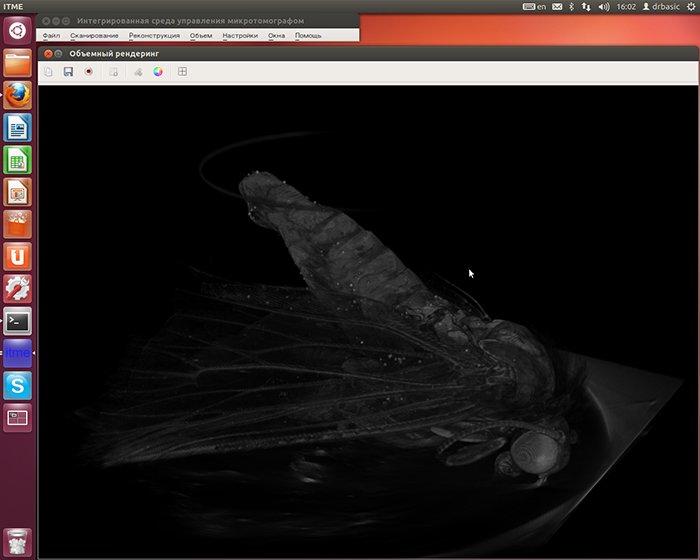
A sufficient frame rate was sustained during the operation by means of a variable level of granularity, as the data is uploaded automatically once the bounding box is shrunk.

Special sets of mathematical functions were implemented to manipulate interface elements in 3D. The initial creation of the section plane, if described in general terms without any formulae, looks like this: a user double-clicks on any point of the model, upon which the point is fixed. Upon further movement of the mouse, it serves as the starting point to display the normal vector to the created plane. However, the plane has already been created in practical terms, lying on the half-line starting from the display coordinates of the mouse cursor and pointing into the depth of field, non-parallel with the perspective lines so that the half-line is projected onto the screen as a point and the plane orientation changes dynamically with movement of the mouse; the user sees it instantly on screen. To finish the creation, the mouse should be clicked one more time to lock the plane's orientation.

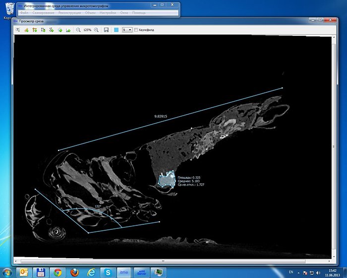
In addition to the elements of model volume manipulation, there are instruments for managing colour spectra of densities and transparency levels.

The self-rendering voxel, the slicing by the section plane and the bounding box were implemented with the help of the VTK (Visualization Toolkit) library functionality.

A list of mathematical functions

1. Plane functions:
   • Plane equation from the normal vector and a point
   • Plane equation from three points
   • Rotation angle of the 2D coordinate system within the plane around the normal vector
   • 2D rectangular area inset within the plane with the benchmark on the normal vector
   • Transition functions from a 2D point within the plane turned around the normal vector to the actual 3D coordinates and inverse transformation
2. Mathematical functions for geometrical calculations:
   • Using a vector to derive two mutually perpendicular vectors, which are also perpendicular to the initial vector
   • Finding a vector perpendicular to the given vector in a 2D system of coordinates
   • Finding the octant from the vector direction and vice versa (finding the vector from the octant)
   • Correcting the central point of the plane for its positioning within the bounding box
   • Determining the inclusion of a point in the box
   • Line–plane intersection
   • Line segment and plane intersection
   • Distance from a point to a line
   • Vector perpendicular to a line from an arbitrary point to a point on the line
   • Distance from point to plane
   • Point-to-plane projection
   • Vector-to-vector projection
   • The angle between 2D vectors
3. Mathematical functions used during reconstruction:
   • Inversion
   • Gamma correction
   • Averaged projection filter
   • The necessary number of anti-aliasing passes
   • Convolution