AmberLight seismic geological modelling

August 3, 2020

AmberLight conducts seismic geological modelling for oil and gas reservoirs based on the interpretation of seismic survey data. The software was created for internal use and for market launch as a more convenient alternative to Roxar RMS. AmberLight builds gridded two-dimensional and three-dimensional geological models with subsequent upload to graphic and text files.

“The company managed to cope with complex tasks in the field of two-dimensional and three-dimensional visualisation, as well as with complex mathematical calculations. The collaboration fee was calculated on the basis of time spent on the project. Detailed technical documentation was developed based on the results of the project.”

Centre for Geological Modelling and Scientific Research of Volga Region

Tabular and graphical results can be used as appendices to the design documentation for the geological exploration work or in the calculation of reserves of oil and gas fields. The geological models can be used in subsequent hydrodynamic modelling.

Description

The graphic part is implemented on .NET WPF, while the algorithmic part uses C++ and is connected to the application as a dynamic library. Raster satellite images are used as a cartographic background for the area under investigation.

Modules:

import/export of data;
visualisation;
map builds;
calculation of isolines.

Types of objects:

points;
polygons;
surfaces;
bitmap image.

In geological modelling, interpolation is used to build maps based on a set of points.

Interpolation methods:

Graphic interface

The main application window is divided into zones.

01	Data tree	A list of folders and subfolders containing a list of objects that can be turned off and on for display by clicking the checkbox to the left of the name. Visible objects will be displayed in all open visualisation windows. Objects inside the tree can be dragged from folder to folder. When dragging one object onto an object of a similar type, the first object will be completely copied into the second one with the name of the latter saved.
02	Visualisation window	Displays sets of points, polygons, bitmap images and surfaces in 2D or 3D.
03	Logs	A window is displayed below, in which text messages are displayed notifying the user of the status and errors.
04	Drop-down menu	In the upper left corner, a drop-down menu contains lists of operations: open, save project, exit application, application information, etc.
05	Toolbar	Icons for quick access to frequently used operations: ‘New project’, ‘Open project’, ‘Save project’.
06	Operation panel	Located on the left. Operations are sorted into categories and are initially hidden. When an object is selected from the data tree, the panel displays the available operations.

The previous 20 project states and user actions are saved. Pressing the Ctrl+Z keyboard shortcut takes the user back to the previous state, while Ctrl+Y returns the user to the next state.

Import

The project begins with data import: the type of object that the engineer wants to import is selected on the tree, then a file is selected in the dialog box.

AmberLight allows users to import a set of points, polygons in XYZ Text format, SUR surface maps, and BMP, JPG, PNG, and TIFF raster images. Data is uploaded in similar formats.

Map builder

The main purpose of the program is to build surfaces in a given area using various interpolation methods based on a set of points identified through seismic exploration.

Delaunay triangulation

Triangulation is an exact interpolation method:

the starting points are connected in such a way that the resulting surface is covered with a ‘patchwork’ of the edges of the triangles;
none of the sides of any triangle intersect with the sides of other triangles;
each triangle is defined by three given points;
the values of the function at the nodes of the regular grid falling within this triangle belong to the plane passing through the vertexes of the triangle.

The method is accurate because the starting points are used to construct triangles and therefore belong to the interpolation function. The triangulation method works best when the set of experimental data contains between 200 and 1,000 points, evenly distributed throughout the area under consideration. Using the Delaunay method to construct an interpolation function from a small number of randomly distributed points leads to the appearance of explicit triangular faces on the surface graph and large rectilinear segments on the isoline map. With large sets of experimental data (> 1,000 points), triangulation becomes very slow. The method is especially effective when it is necessary to preserve the lines of surface breaks.

Nearest neighbour interpolation

The simplest interpolation method, where the nearest known value is selected as the target value. Designed primarily for testing and validating other interpolation methods.

Kriging interpolation

The most popular method in geostatistics is the linearly weighted moving average. The weight, however, depends not only on the distance, but also on the direction and orientation of the neighbouring data at the point of calculation.

Multilevel B-spline interpolation

An algorithm in which a surface is formed to different levels of detail. This is a very quick method. Thanks to the extrapolation inherent in splines it shows good results on smooth surfaces, especially in areas without data. The resulting surface may not pass through the grid nodes, though it is smooth and twice differentiable throughout the modelling area. Furthermore, the method is relatively simple to implement and builds surfaces that look realistic when compared with the original data. The result may not be perfect when the source data contains noise, however.

Object statistics

After calculating the statistics, the user can build maps with a bounded coordinate interval to exclude deliberately erroneous data. For each type of object, the set of calculated indicators is different.

For a set of points:

total number of points in the set;
average value of Z;
maximum and minimum values for the X, Y and Z coordinates of the point.

For polygons:

total number of points;
minimum and maximum values for each coordinate of the point;
average value of Z;
the number of polygons (broken lines) inside the object;
the sum of the lengths of all polygons within a given object;
area of all closed polygons – where the first and last points coincide.

For surfaces:

number of nodes;
minimum and maximum values of the X, Y and Z coordinates;
average value of Z;
area;
volume.

Surface operations

Operations with two surfaces were implemented.

01	Mathematical	An operation is performed on each Z coordinate (applicate) of each point on surface A using the value of the applicate of a point with the same coordinates (X, Y, Z) on surface B. Possible operations: A = A + B; A = A − B; A = A × B; A = A / B; A = B.
02	Conditional	The value of the Z coordinate of a point on surface A is equal to the value of the Z coordinate of a point on surface B if the condition is met. Possible conditions: A > B; A < B.
03	Destructive	Removes the nodes of surface A if the condition is met. Possible conditions: A > B; A ≥ B; A < B; A ≤ B.

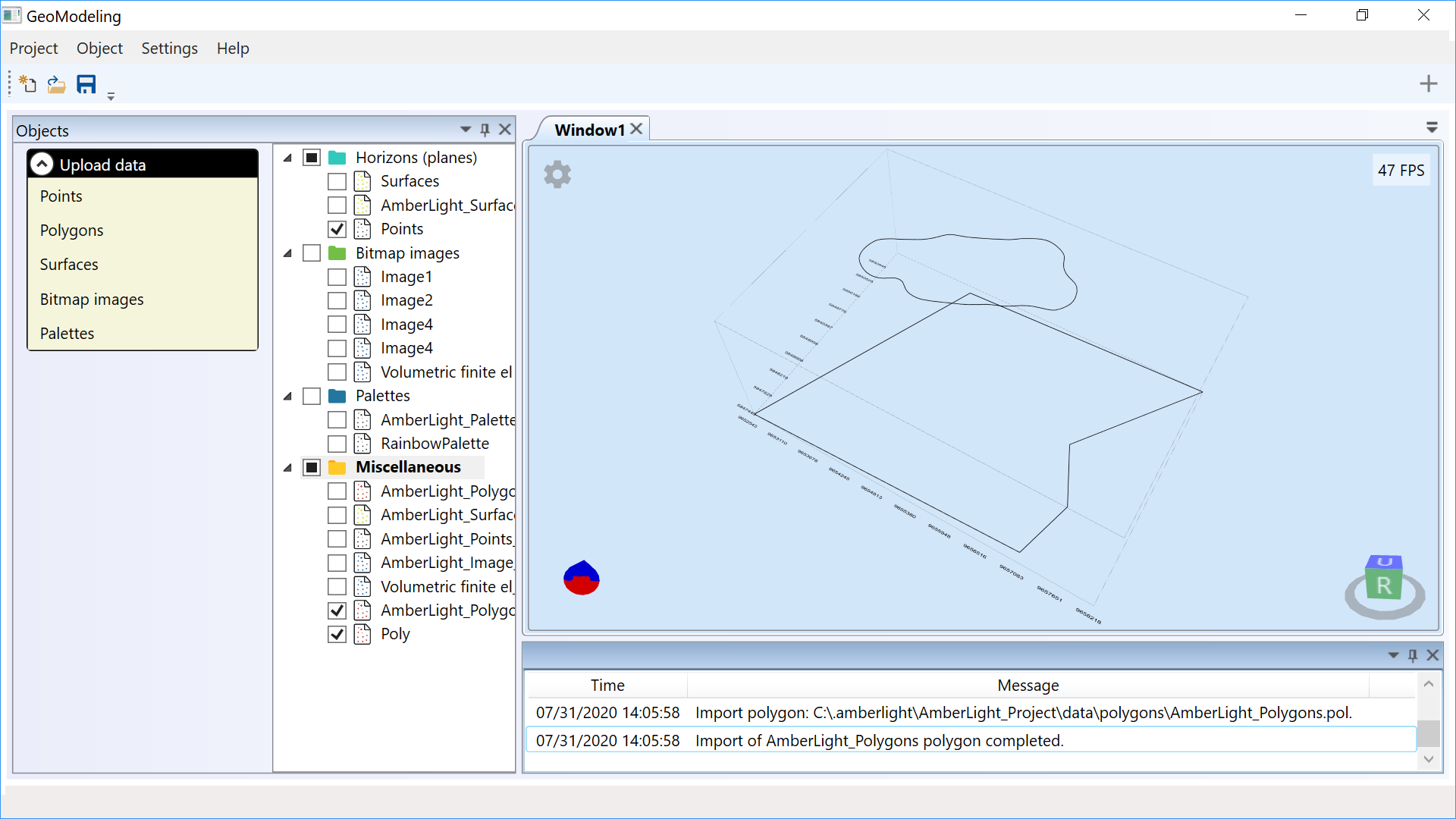
Logical operations can be applied to the surface and the polygon if the polygon is closed. The calculation uses the X and Y coordinates:

removal of all points outside the polygon;
removal of all points inside the polygon;
setting Z coordinate as equal to a given constant for all points outside the polygon;
setting Z coordinate as equal to a given constant for all points inside the polygon.

Visualisation

Modes for displaying objects:

2D – two-dimensional visualisation;
3D – three-dimensional visualisation.

Visualisation windows can be opened using a special button. By default, if there are no windows yet, a 2D view window is created.

When the first object appears, the window is adjusted so that the whole object is placed in the centre, with free space at the edges equal to 1/10 of the total size of the window. When an object in the tree is selected, it is displayed in all open visualisation windows.

The object with the highest Z coordinate value is located above the others (it is displayed on top of the other objects). When two surfaces intersect, the closer part of the surfaces is drawn, and the farther part is hidden. If the point or polygon lies below the rendered surface, then it does not appear.

Depending on the settings, bitmaps are drawn behind or on top of all other objects. The degree of transparency can be set so that the objects that are farther away are not completely hidden when displayed.

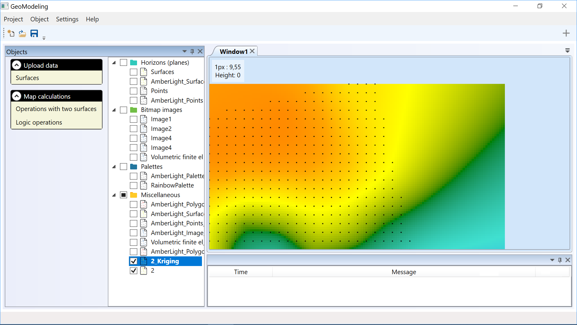
Multiple source files can be displayed. Changes to the colour palette of the surface, raster image transparency etc. are implemented ‘on the fly’. Pressing Ctrl and the left mouse button allows the user to identify the height at any given point on the surface, and the keyboard shortcut Ctrl + F directs the ‘camera’ to the selected object in the tree.

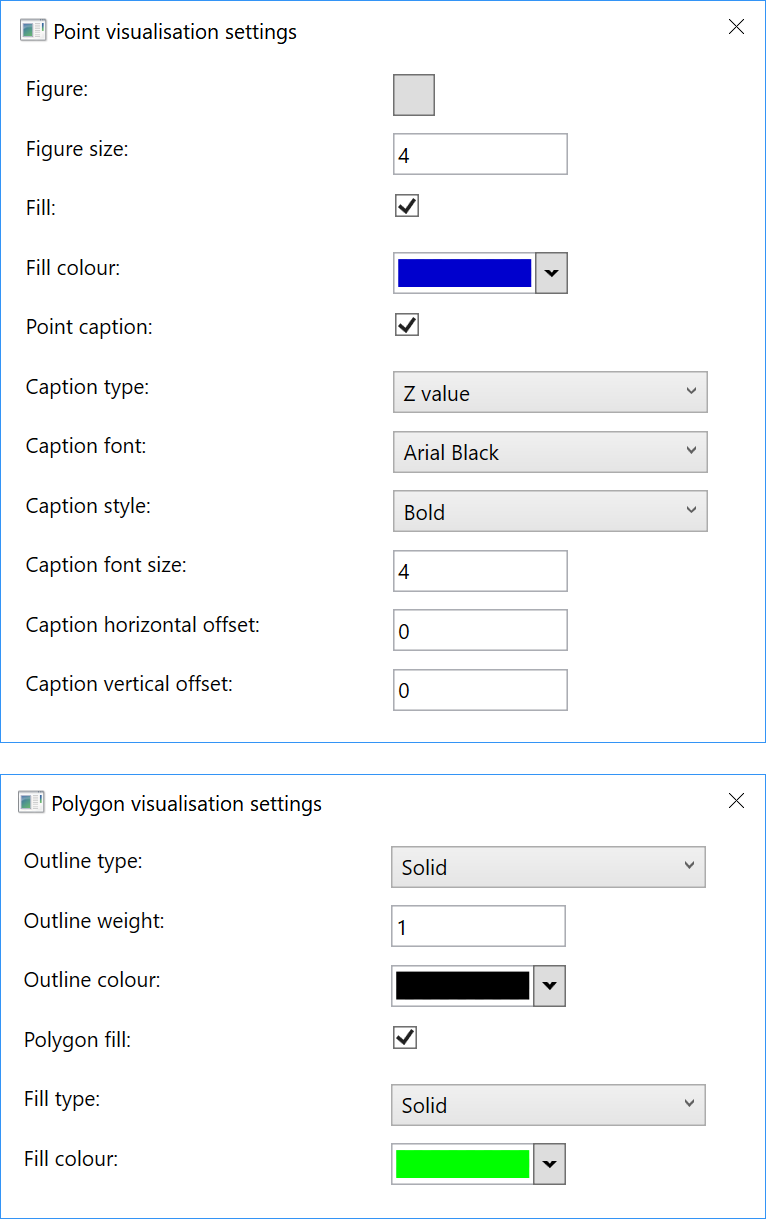
The bitmap object is assigned coordinates to snap the raster and prevent shifting when zooming. Each object has its own visualisation settings.

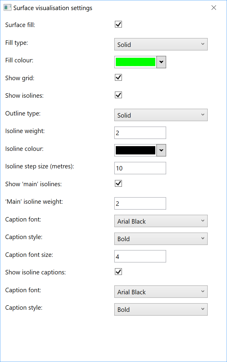
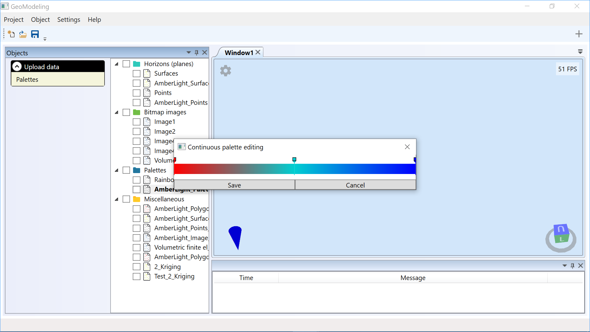
To customise surface displays, the program recommends setting up a discrete or continuous palette.

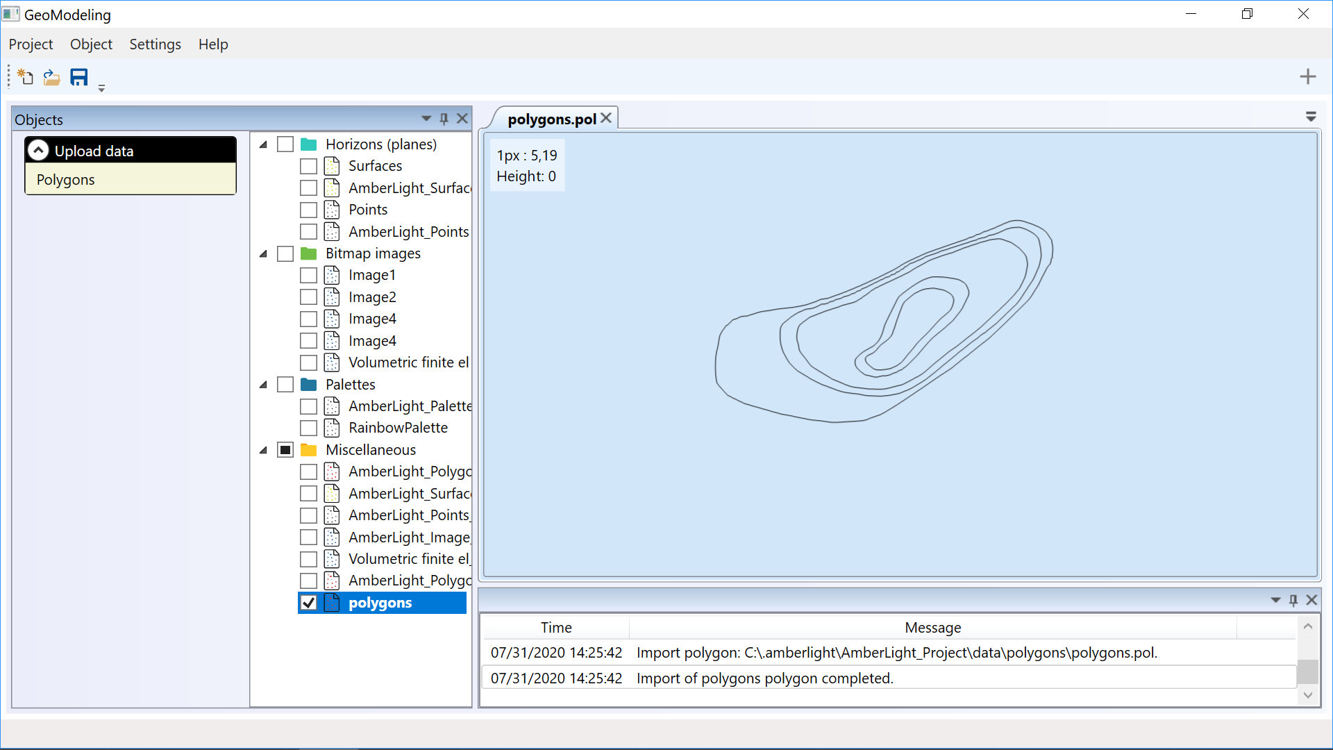
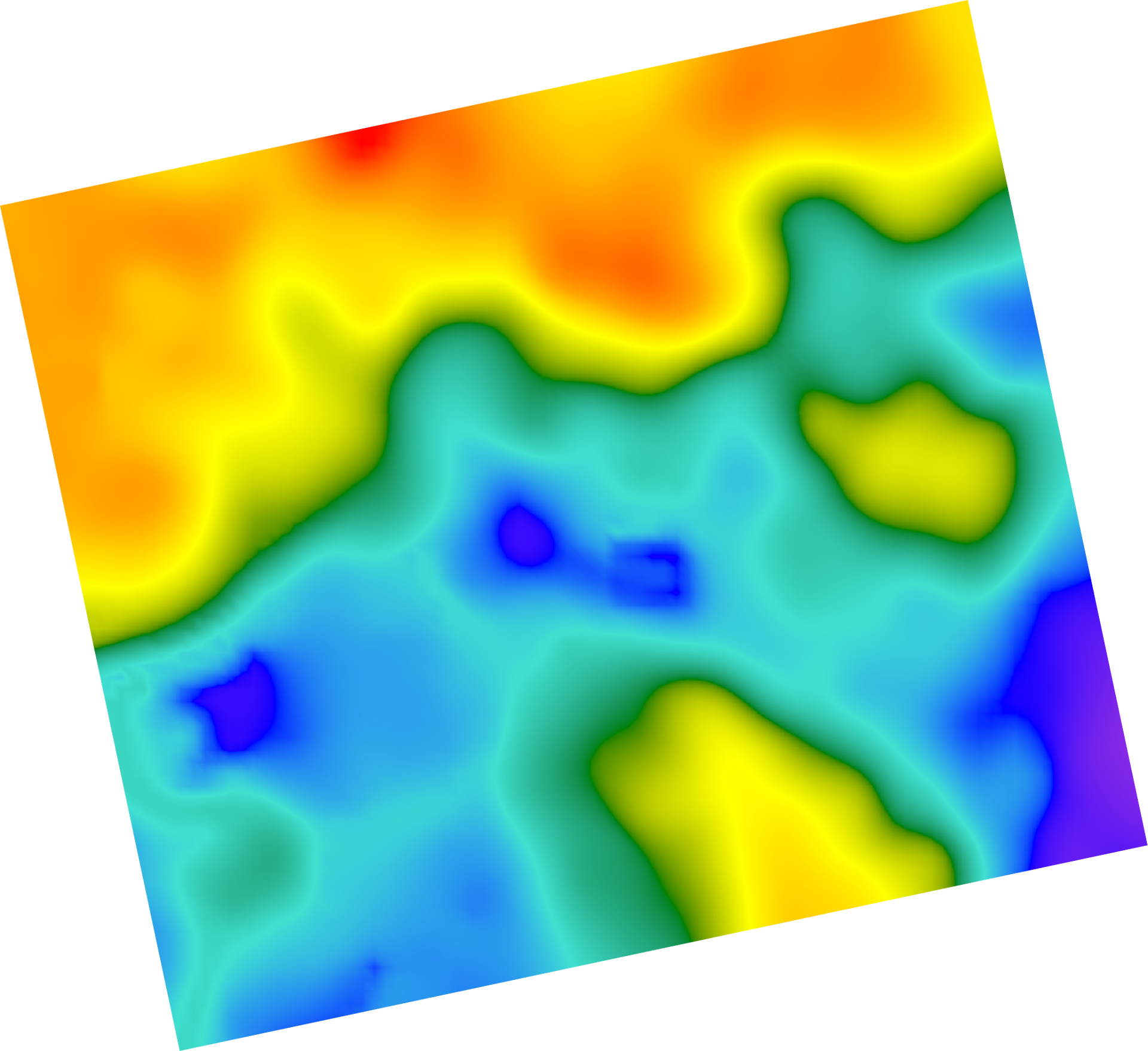
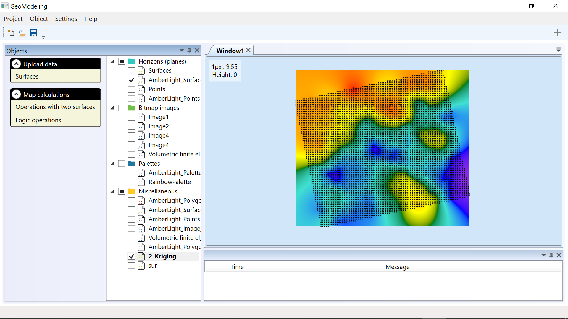
2D visualisation displays raster images, points, polygons and surfaces in the horizontal plane. Component logic is implemented from scratch by means of .NET WPF. When zooming in or moving objects, only the visible parts of the objects are drawn.

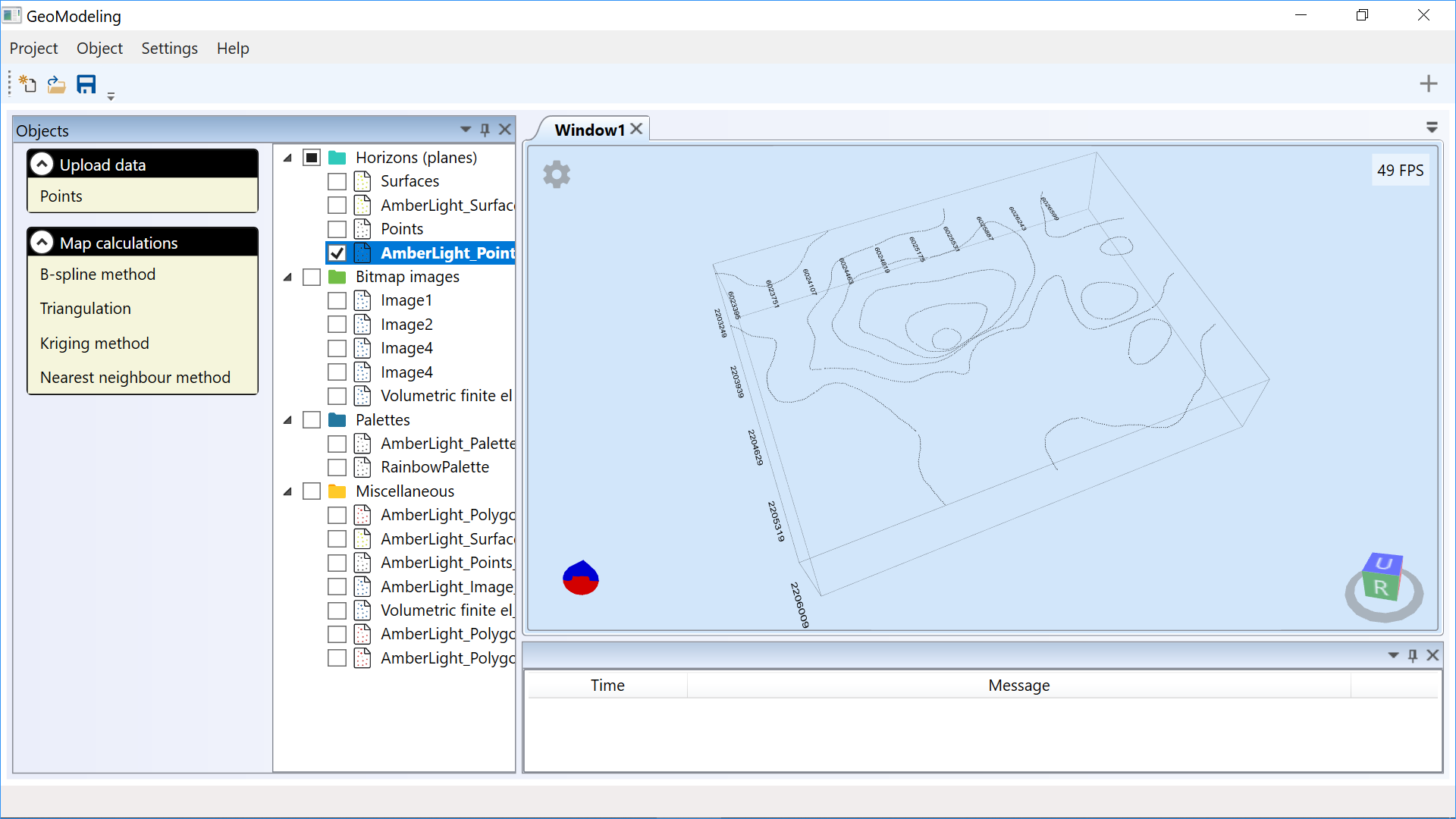
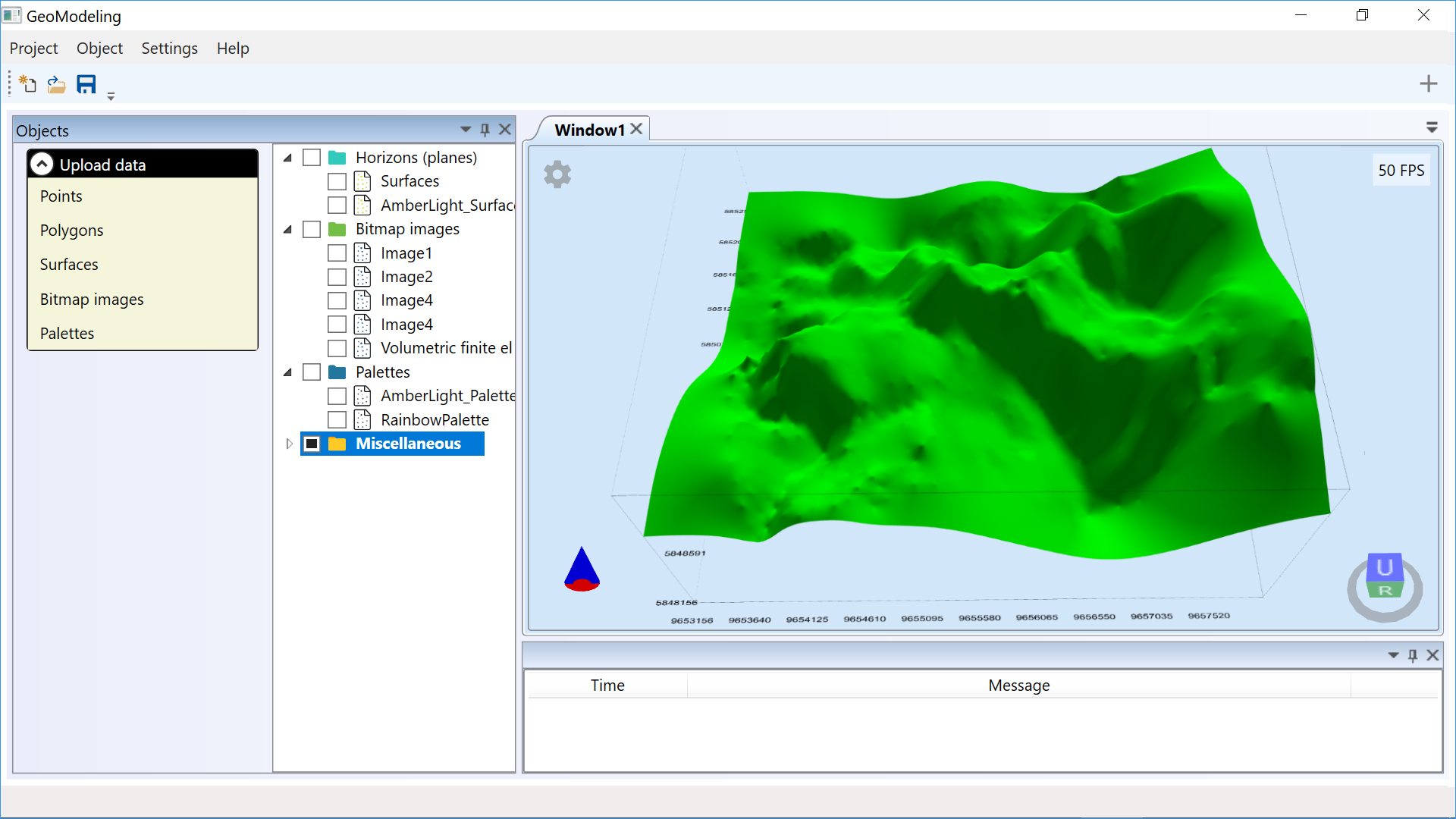
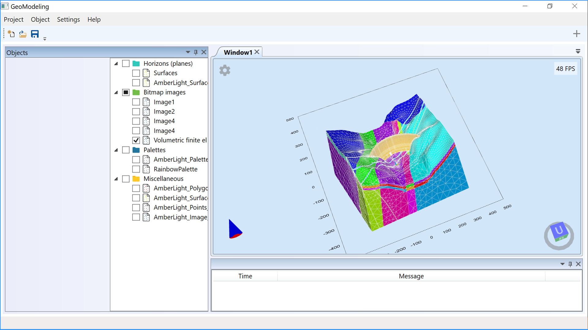
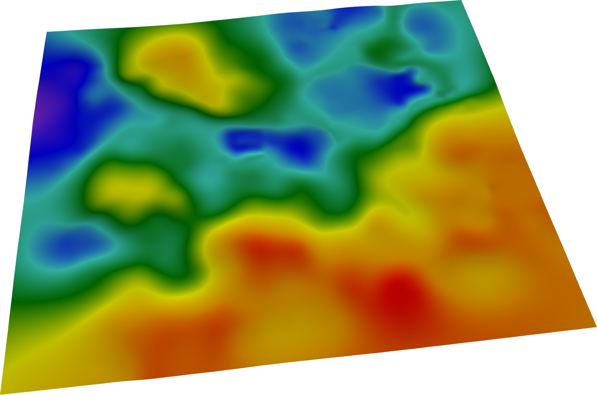
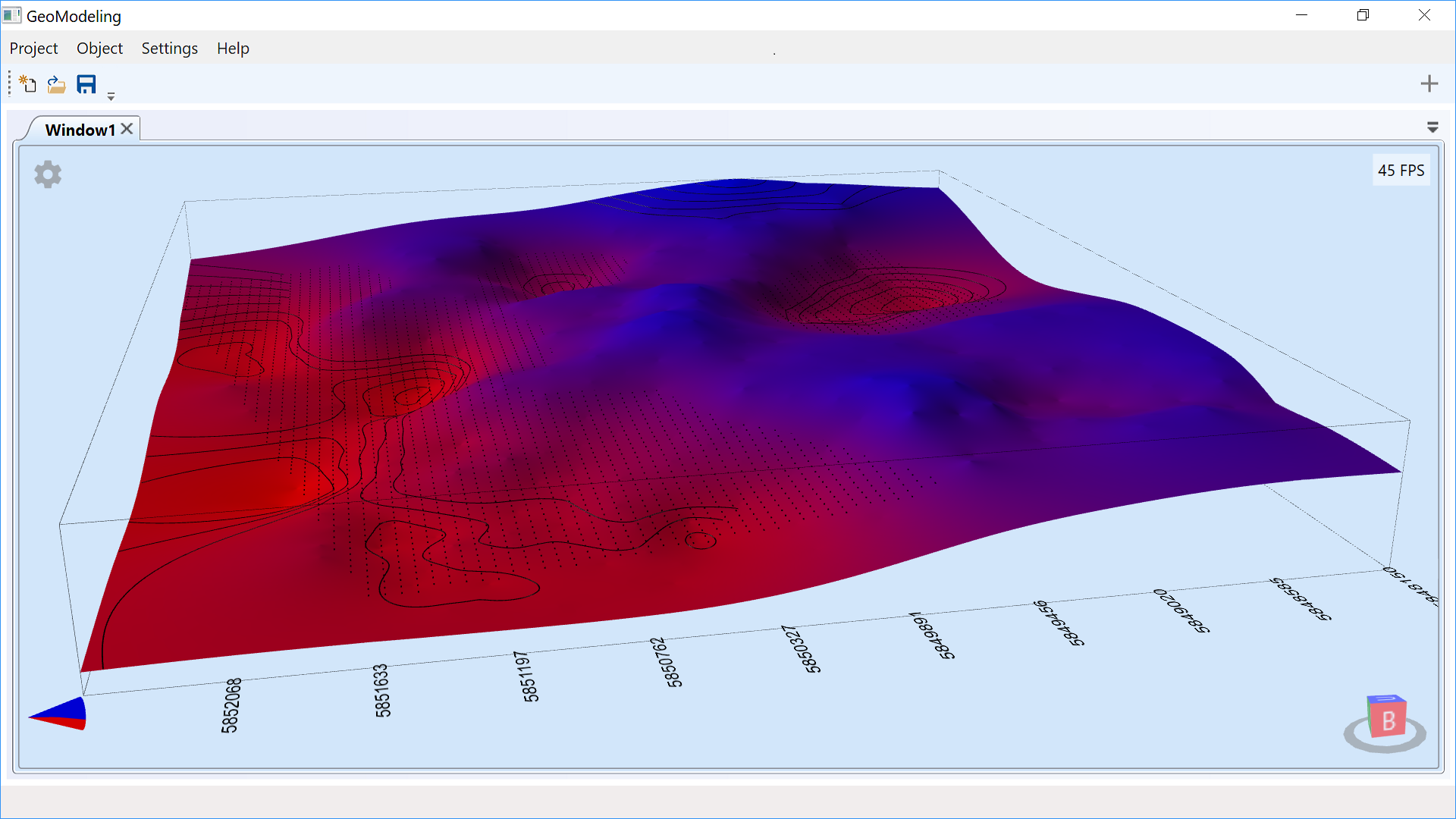
For 3D visualisation, a grid is drawn. One of three types of light source can be selected: solar, three-point, or standard.

An arrow is displayed in the lower left corner, which rotates with all objects and points to the north, in the direction of increasing ordinates (Y coordinate). The lower part of the arrow (in the direction of the decreasing Z coordinate) is coloured red, and the upper part (in the direction of the increasing Z coordinate) is coloured blue.

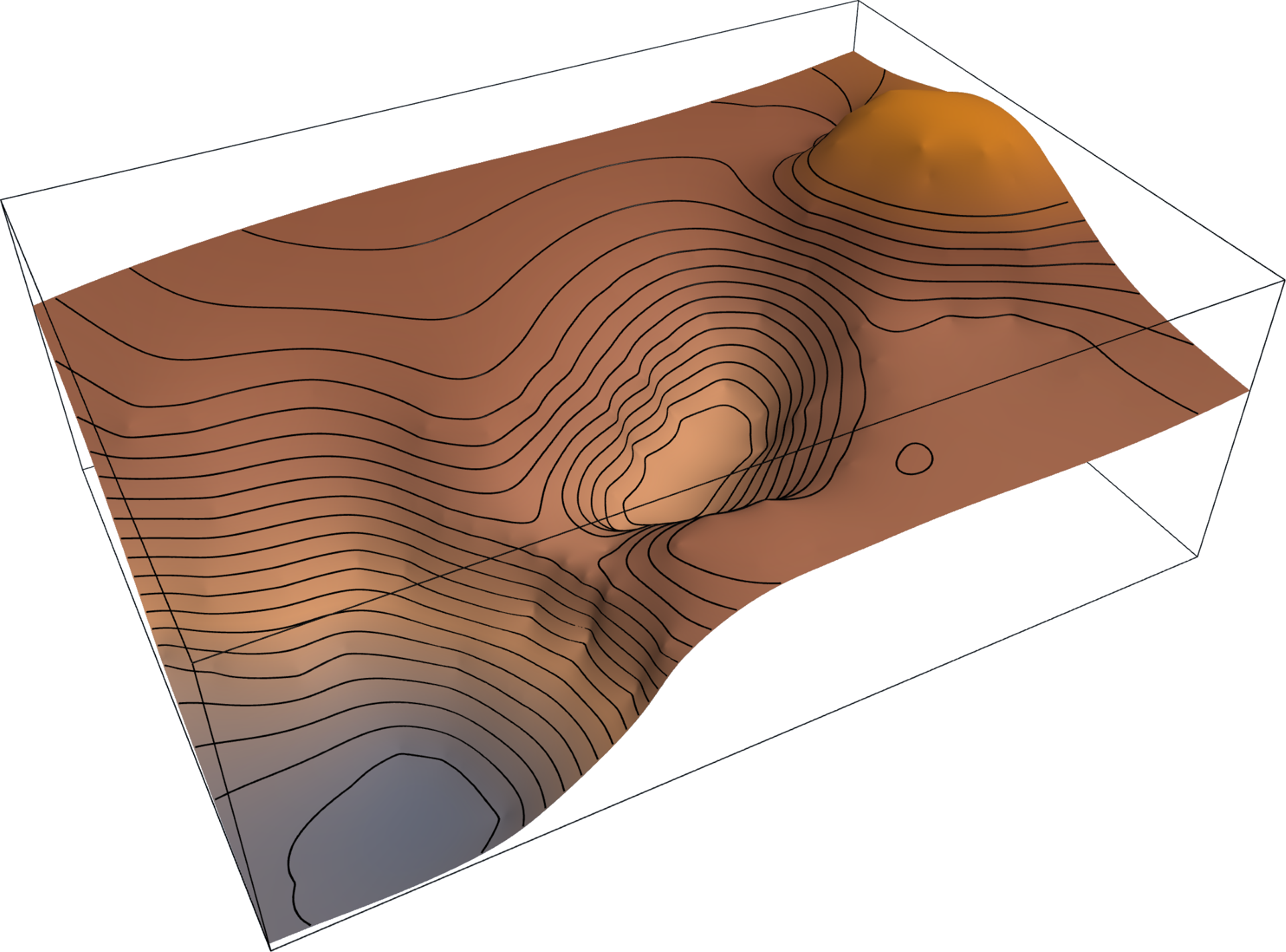
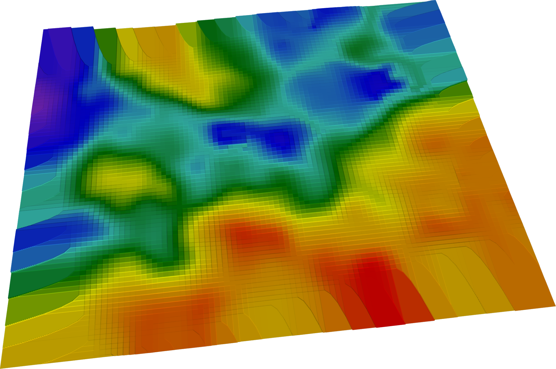
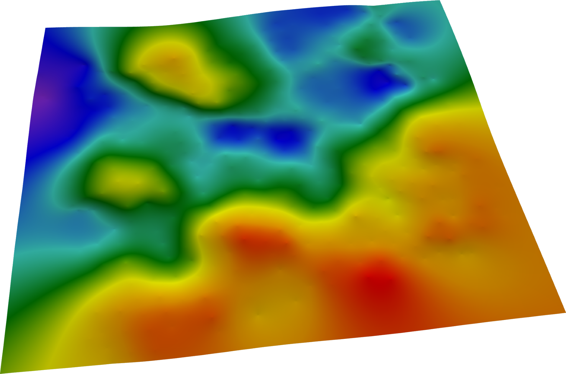
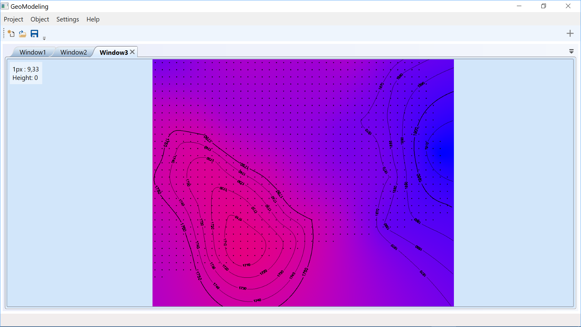
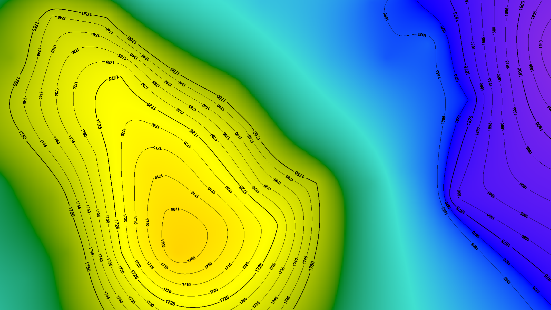
Isoline calculation

Isolines are surface lines with identical height value. Isolines make it possible to visualise flat and angular objects. The closer the isolines are to each other, the greater the curvature of the surface.

Based on the minimum and maximum surface heights and the step size specified in the settings, a set of heights at which isolines will be drawn is calculated. Then, at each height level, a set of isolines is calculated using the marching squares algorithm.

.NET Algorithm C++ CAD Desktop GPS Interface WPF